Differential expression between clusters using scde
Preprocessed data
Note: Similarly to the identification of markers for each cluster, this analysis uses data prepared identically to the differential expression between experimental groups using scde:
- ERCC spike-in features are removed,
- Cells in the data set is subsetted by time point,
- Genes in the data set are subsetted for those detected at sufficient levels within each time point,
- Error models are computed on the subsetted data sets
In addition, this analysis diverges from the differential expression between supervised experimental groups by consideration of unsupervised clusters identified within each time point.
Differential expression
Setup
Let us first define a list to store the result tables returned by scde:
scde.res <- list()In addition, note that several functions defined in the first scde section will be re-used here.
Contrasts
2h (2 vs 3)
Identification of unsupervised clusters at 2h p.i. revealed that cluster 2 and 3 to comprise exclusively stimulated and majoritarily uninfected DCs, respectively. However, both clusters display some degree of overlap between their markers genes. Thus, a direct comparison of the two unsupervised clusters may detect more subtle differences and effect sizes:
groupTarget <- 2; groupRef <- 3
sg.test <- factor(sce.ifm.2h$quickCluster.2h, levels = c(groupTarget, groupRef))
names(sg.test) <- colnames(sce.ifm.2h); summary(sg.test)
contrastName <- sprintf("2h_cluster%s-cluster%s", groupTarget, groupRef); message(contrastName)
stopifnot(all(rownames(o.ifm.2h) == colnames(cd.ifm.2h)))
scde.res[[contrastName]] <- scde.expression.difference(
    o.ifm.2h, cd.ifm.2h, o.prior.2h, sg.test, n.cores = 4, verbose = 1
  )
2h (2 vs 1)
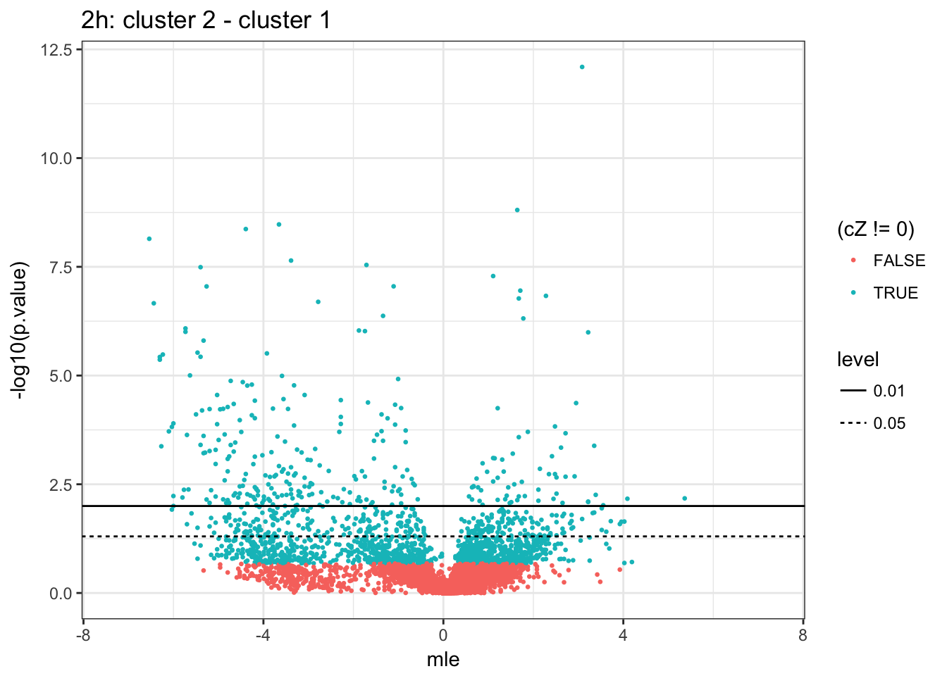
In addition, cluster 2 (exclusively stimulated) may also be compared directly to cluster 1, the latter displaying a large and even representation of uninfected and challenged cells. Again, a direct comparison of the two unsupervised clusters may detect subtle differences and effect sizes:
groupTarget <- 2; groupRef <- 1
sg.test <- factor(sce.ifm.2h$quickCluster.2h, levels = c(groupTarget, groupRef))
names(sg.test) <- colnames(sce.ifm.2h); summary(sg.test)
contrastName <- sprintf("2h_cluster%s-cluster%s", groupTarget, groupRef); message(contrastName)
stopifnot(all(rownames(o.ifm.2h) == colnames(cd.ifm.2h)))
scde.res[[contrastName]] <- scde.expression.difference(
    o.ifm.2h, cd.ifm.2h, o.prior.2h, sg.test, n.cores = 4, verbose = 1
  )
4h (2 vs 1)
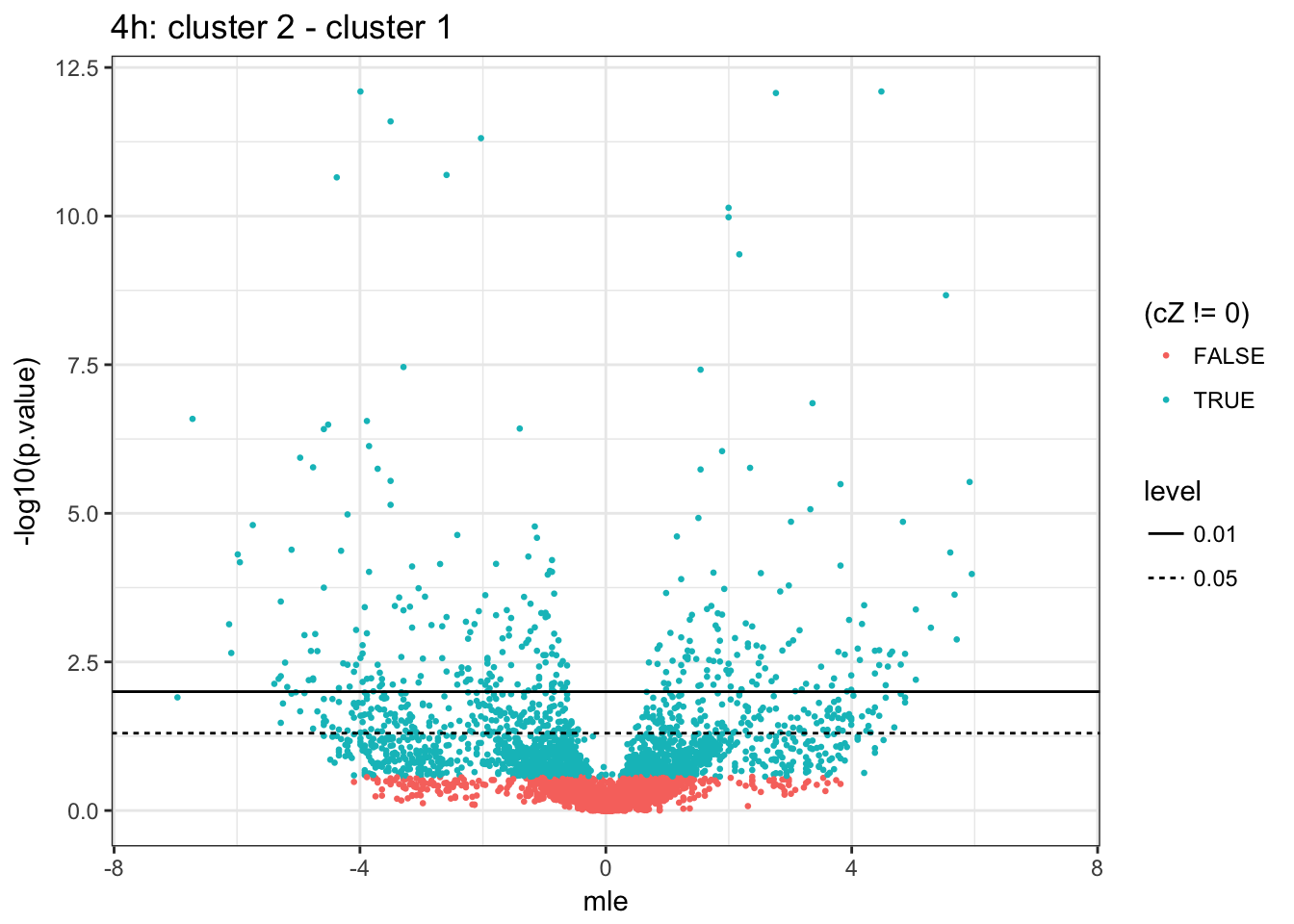
At 4h p.i., unsupervised clusters reveals a marked distinction between exposed and infected DCs, accounting for the majority of clusters 2 and 1, respectively, irrespective of the infection. Thus, a direct comparison of the two unsupervised clusters may detect more subtle differences and effect sizes:
groupTarget <- 2; groupRef <- 1
sg.test <- factor(sce.ifm.4h$quickCluster.4h, levels = c(groupTarget, groupRef))
names(sg.test) <- colnames(sce.ifm.4h); summary(sg.test)
contrastName <- sprintf("4h_cluster%s-cluster%s", groupTarget, groupRef); message(contrastName)
stopifnot(all(rownames(o.ifm.4h) == colnames(cd.ifm.4h)))
scde.res[[contrastName]] <- scde.expression.difference(
    o.ifm.4h, cd.ifm.4h, o.prior.4h, sg.test, n.cores = 4, verbose = 1
  )
6h (2 vs 1)
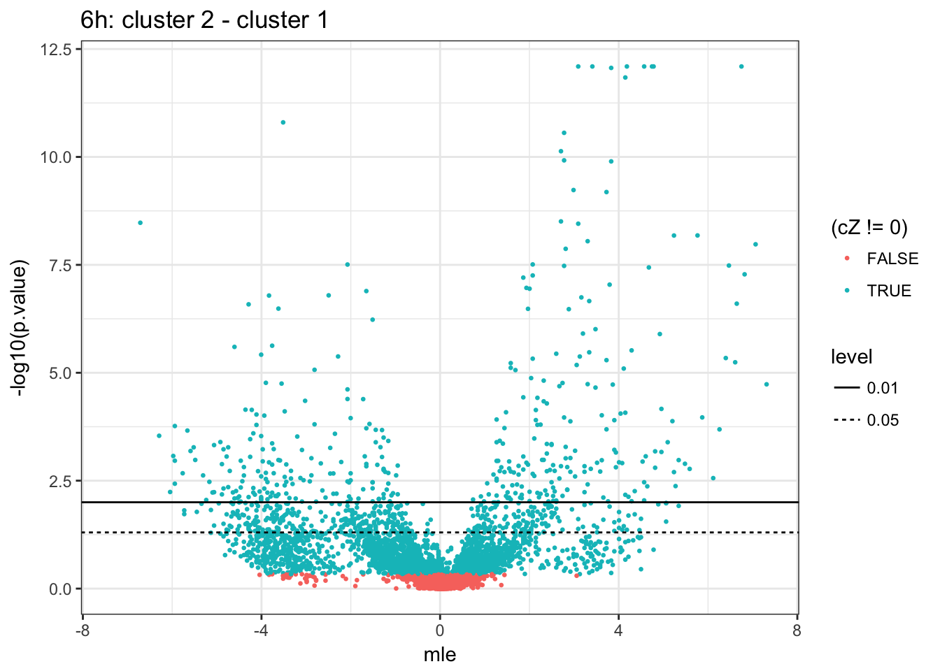
At 4h p.i., unsupervised clusters reveals a notable under-representation of STM-D23580 exposed DCs in cluster 1 relative to cluster 2, in contrast to STM-LT2 exposed DCs showing the opposite trend. Thus, a direct comparison of the two unsupervised clusters may detect more subtle differences and effect sizes:
groupTarget <- 2; groupRef <- 1
sg.test <- factor(sce.ifm.6h$quickCluster.6h, levels = c(groupTarget, groupRef))
names(sg.test) <- colnames(sce.ifm.6h); summary(sg.test)
contrastName <- sprintf("6h_cluster%s-cluster%s", groupTarget, groupRef); message(contrastName)
stopifnot(all(rownames(o.ifm.6h) == colnames(cd.ifm.6h)))
scde.res[[contrastName]] <- scde.expression.difference(
    o.ifm.6h, cd.ifm.6h, o.prior.6h, sg.test, n.cores = 4, verbose = 1
  )
Volcano plots
Let us first identify the extreme values of maximum likelihood estimate of fold-change to scale subsequent plot for comparability:
mleRange <-
  max(abs(do.call("c", lapply(scde.res, function(x){return(x$mle)}))))*c(-1,1)
pRange <- c(
    0,
    -log10(min(do.call("c", lapply(scde.res, function(x){
      return(convert.z.score(x)$p.value)
    }))))
)
2h (2 vs 1)
4h (2 vs 1)
6h (2 vs 1)
Count DE genes at various cut-offs
2h (2 vs 1)
| P.01 | P.05 | cZ | |
|---|---|---|---|
| 2h: cluster2 - cluster1 | 272 | 580 | 1613 |
4h (2 vs 1)
| P.01 | P.05 | cZ | |
|---|---|---|---|
| 4h: cluster2 - cluster1 | 293 | 634 | 2000 |
6h (2 vs 1)
| P.01 | P.05 | cZ | |
|---|---|---|---|
| 6h: cluster2 - cluster1 | 369 | 798 | 3512 |