Sample-level quality control
Plotting themes
First of all, let us define:
- theme elements used throughout various figures in the following sections:
sampleQCtheme <-
  theme_minimal() +
  theme(
    axis.ticks.x = element_blank(), axis.text.x = element_blank(),
    panel.grid.major.x = element_blank(),
    panel.grid.minor = element_blank(),
    legend.position = "bottom", legend.box = "vertical")
groupQCtheme <-
theme_bw() +
theme(
axis.text.x = element_text(angle=90, hjust = 1, vjust = 0.5, size = rel(0.6)),
legend.position = "bottom", legend.box = "vertical",
panel.grid.minor = element_blank(),
plot.title = element_text(hjust = 0.5)
)- a set of colours used to indicate phenotype information consistently across the subsequent figures:
col.time <- brewer.pal(9, "Set3")[c(2,7:8)]
col.infection <- brewer.pal(12, "Paired")[c(9,4,2,5)]
col.status <- brewer.pal(12, "Paired")[c(9,1,7,3,5)]
names(col.time) <- levels(sce.all$Time)[1:3]
names(col.infection) <- levels(sce.all$Infection)
names(col.status) <- levels(sce.all$Status)- let us also initialise a
data.framethat will be used to store outliers identified in each of the quality control filters defined below:
outliers <- data.frame(row.names = colnames(sce.sc))Blanks
Blank samples are designed to detect major technical issues during library preparation; in particular contamination, as only ERCC spike-in features are expected in those samples.
The scater calculateQCMetrics method may then be used to calculate the relevant QC metrics:
sce.blank <- calculateQCMetrics(
  sce.blank,
  exprs_values = "counts",
  feature_controls = list(ERCC = isSpike(sce.blank, "ERCC"))
)
## Warning in calculateQCMetrics(sce.blank, exprs_values = "counts",
## feature_controls = list(ERCC = isSpike(sce.blank, : spike-in set 'ERCC'
## overwritten by feature_controls set of the same name## Note that the names of some metrics have changed, see 'Renamed metrics' in ?calculateQCMetrics.
## Old names are currently maintained for back-compatibility, but may be removed in future releases.In the SingleCellExperiment object augmnented by QC metrics, let us visualise the most abundant features which displays the expected over-representation of ERCC spike-in features:
plotHighestExprs(sce.blank, n = 100)![]()
FastQC / MultiQC
GC content (FastQC)
GC content is species-specific; it can be estimated from the annotated transcriptome or the sequenced data. Therefore, GC content excessively different from the majority of samples can indicate issues during library preparation or contamination.
Let us identify as outliers single cells that display a GC content excessively different from the median of single cell samples, here beyond 3 MADs:
outliers$GC <- isOutlier(sce.sc$FastQC_percent_gc, 3)
table(outliers$GC)
##
## FALSE TRUE
## 372 1Let us visualise outliers, along with blank and bulk samples for reference:
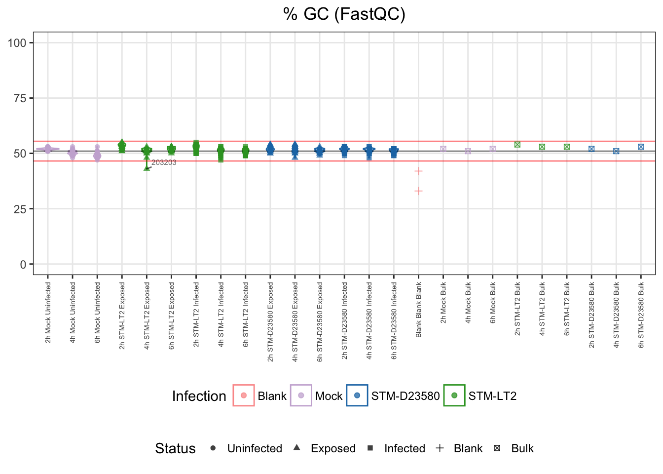
For reference:
- single cells
- median: 51%
- cut-offs
- upper bound: 55%
- lower bound: 47%
Alignment rate (HISAT2)
Technical issues introduced during library preparation may result in an excessively low alignment rate. Nevertheless, libraries with slightly lower alignment rates may still yield a library size comparable to the majority of samples.
For those reasons reasons, let us identify as outliers single cells with an alignment rate excessively lower than the median of single cell samples, here beyond 3 MADs:
outliers$AlignedPercent <- isOutlier(sce.sc$Bowtie.2_overall_alignment_rate, 3, "lower")
table(outliers$AlignedPercent)
##
## FALSE TRUE
## 353 20Let us visualise outliers, along with blank and bulk samples for reference:
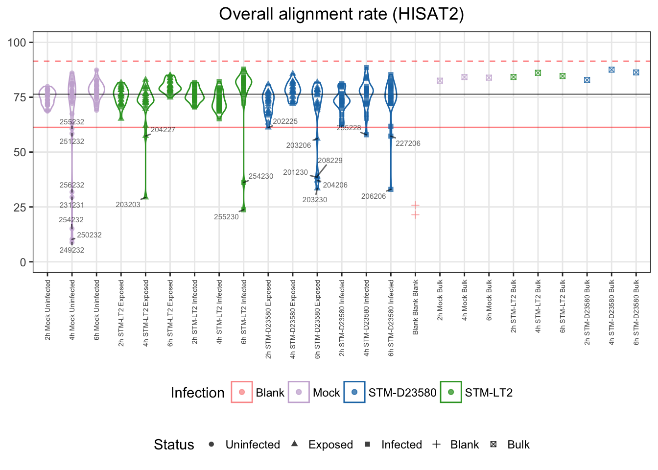
For reference:
- single cells
- median: 76%
- cut-off
- lower bound: 61%
Assigned reads / Library size (featureCounts)
An excessively small count of aligned reads assigned to annotated genomics features (i.e., library size) may indicate technical issues during library preparation or low quality samples. Moreover, library size excessively different from the majority of samples may introduce bias due to under- or over-sampling of RNA fragments, and negatively affect the performance of between-sample normalisation algorithms.
Let us identify as outliers single cells with a count of assigned read pairs (i.e. library size) excessively different from the median of single cell samples, here beyond 3 MADs:
outliers$AssignedCount <- isOutlier(sce.sc$featureCounts_Assigned, 3, log = TRUE)
table(outliers$AssignedCount)
##
## FALSE TRUE
## 352 21Let us visualise outliers, along with blank and bulk samples, for reference:
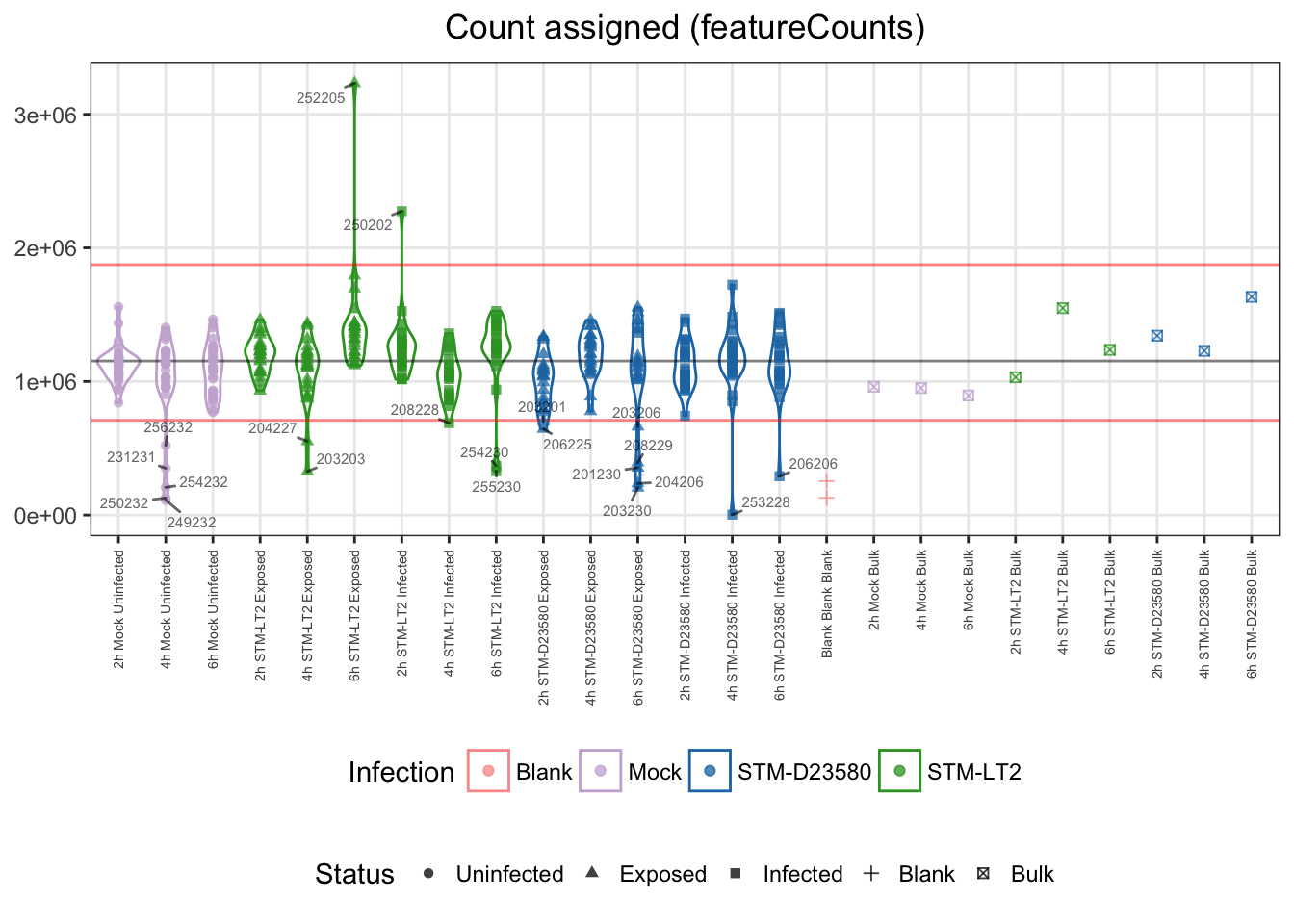
For reference:
- single cells
- median: 1.2e+06
- cut-offs
- lower bound: 0.7e+06
- upper bound: 1.9e+06
Percentage assigned (featureCounts)
Similarly, unusually low assignment rate of reads to annotated genomic features may indicate technical issue; for instance during poly-A selection.
Let us identify as outliers single cells with a rate of assigned reads excessively lower than the median of single cell samples, here beyond 3 MADs:
outliers$AssignedPercent <- isOutlier(sce.sc$featureCounts_percent_assigned, 3)
table(outliers$AssignedPercent)
##
## FALSE TRUE
## 357 16Let us visualise outliers, along with blank and bulk samples, for reference:
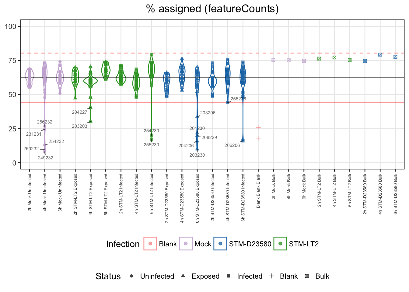
For reference:
- single cells
- median: 62%
- cut-off
- lower bound: 44%
Summary
Let us display the count of cells identified as outliers for each of the filters so far:
fastqc.fr <- FilterRules(colnames(outliers))
fastqc.fr
## FilterRules of length 4
## names(4): GC AlignedPercent AssignedCount AssignedPercent| Fail | Pass | |
|---|---|---|
| 373 | 373 | |
| GC | 1 | 372 |
| AlignedPercent | 20 | 353 |
| AssignedCount | 21 | 352 |
| AssignedPercent | 16 | 357 |
| 1 | 347 |
Note: In the above table, the first row simply indicates the total count of cells before any filtering; conversely, the last row indicates the count of cells that failed or passed, respectively, all filters.
scater
Calculation of QC metrics
The following sections require the estimation of several QC metrics that leverage control features and control samples, as means to identify outliers among single cells.
Let us apply the scater calculateQCMetrics to calculate the relevant QC metrics in the single cell data set, using set of spike-in control features:
sce.sc <- calculateQCMetrics(
  sce.sc,
  feature_controls = list(
    ERCC = isSpike(sce.sc, "ERCC"),
    MT = as.logical(seqnames(sce.sc) == "MT")
  )
)
## Warning in calculateQCMetrics(sce.sc, feature_controls = list(ERCC =
## isSpike(sce.sc, : spike-in set 'ERCC' overwritten by feature_controls set
## of the same name## Note that the names of some metrics have changed, see 'Renamed metrics' in ?calculateQCMetrics.
## Old names are currently maintained for back-compatibility, but may be removed in future releases.For reference purpose in upcoming figures, let us also calculate the relevant QC metrics in the complete data set:
sce.all <- calculateQCMetrics(
  sce.all,
  feature_controls = list(
    ERCC = isSpike(sce.sc, "ERCC"),
    MT = as.logical(seqnames(sce.sc) == "MT")
  ),
  cell_controls = list(
    Bulk = which(sce.all$Status == "BULK"),
    Blank = which(sce.all$Status == "Blank")
  )
)
## Warning in calculateQCMetrics(sce.all, feature_controls = list(ERCC =
## isSpike(sce.sc, : spike-in set 'ERCC' overwritten by feature_controls set
## of the same name## Note that the names of some metrics have changed, see 'Renamed metrics' in ?calculateQCMetrics.
## Old names are currently maintained for back-compatibility, but may be removed in future releases.Library size
The library size refers to the total count of reads assigned to annotated features in each individual sample.
Here, let us simply show the direct relation between log10_total_counts computed by calculateQCMetrics and the featureCounts_Assigned counts detected by MultiQC in an earlier section above:
with(
  data.frame(colData(sce.sc)),
  all(abs(log10_total_counts == log10(featureCounts_Assigned+1)))
)
## [1] TRUEAs a result, this metric is identical to the featureCounts_Assigned metric described above; and thereby would unnecessarily identify the same outliers.
Library complexity
Library complexity refers to the proportion of assigned reads accounted for by the \(N\) most abundant features within each individual sample, with values for \(N\) usually ranging from tens to hundreds. It is expected to observe a lower library complexity in single cells relative to bulk samples, due to higher dropout events in single cells, and the union of multiple phenotypes within bulk samples. In contrast, blank samples are expected to have extremely low library complexity, as only up to 92 ERCC spike-ins sequences are expected in those libraries, in contrast to thousands of genomic features in biological samples.
In the SingleCellExperiment object augmnented by QC metrics, let us visualise the library complexity profile against experimental phenotype information:
plotScater(
  sce.all, block1 = "Status", block2 = "Infection",
  colour_by = "Time", nfeatures = 300, exprs_values = "counts"
)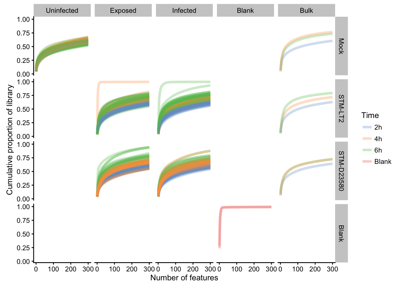
First, from a QC perspective:
- Blank samples show a very low library complexity, as expected.
- Bulk samples show a generally high library complexity, as expected.
- Single cells generally show a complexity profile comparable to that of bulk samples, indicative of healthy dendritic cells and unbiased sampling of diverse transcripts.
- A small subset of single cells (e.g.,
exposed:D23580:6h,exposed:LT2:4h,infected:D23580:4h,infected:D23580:6h,infected:LT2:6h) show suspiciously low library complexity; suggestive of technical issues during library prepration (e.g., amplification bias, dropout events). Those single cells must therefore be treated as outliers, and be removed from the data set prior to feature selection, normalisation, and subsequent analyses.
Now, from a biological perspective, interesting observations may be made:
- Library complexity seems to decrease with
Timeinexposedandinfectedsamples in cells exposed to or infected by bacteria, in contrast to control uninfected cells. This may indicate a polarisation of single cells toward specialised phenotype(s) after infection or exposure (e.g., cytokine production, antigen presentation). Mock(i.e.,uninfected) single cells tend to show a consistent, relatively high library complexity- Both
LT2andD23580infections show a gradual decrease of library complexity over time. This observation might be more pronounced forD23580.
Most abundant features
Although abundantly expressed features are an expected aspect of cell biology (e.g., myosin in muscle cells, clusters of differentiation in immune cells) which may contribute to the identification and classification of cell types, overly abundant features in RNA-Seq libraries may indicate issues during library preparation; in particular, cDNA amplification bias. Moreover, when a small number of highly abundant features account for an excessive proportion of sequenced reads, expression levels for the vast majority of other genes may not be estimated with sufficient accuracy.
Identification
Let us identify as outliers single cells in which the 50, 100, and 200 most abundant features account for a proportion of library size excessively higher than the median of single cell samples, here beyond 3 MADs:
Top 50
outliers$top50 <- isOutlier(sce.sc$pct_counts_top_50_features, 3)
table(outliers$top50)
##
## FALSE TRUE
## 367 6Top 100
outliers$top100 <- isOutlier(sce.sc$pct_counts_top_100_features, 3)
table(outliers$top100)
##
## FALSE TRUE
## 367 6Top 200
outliers$top200 <- isOutlier(sce.sc$pct_counts_top_200_features, 3)
table(outliers$top200)
##
## FALSE TRUE
## 367 6Visualisation
Let us visualise outliers, along with blank and bulk samples, for reference:
50
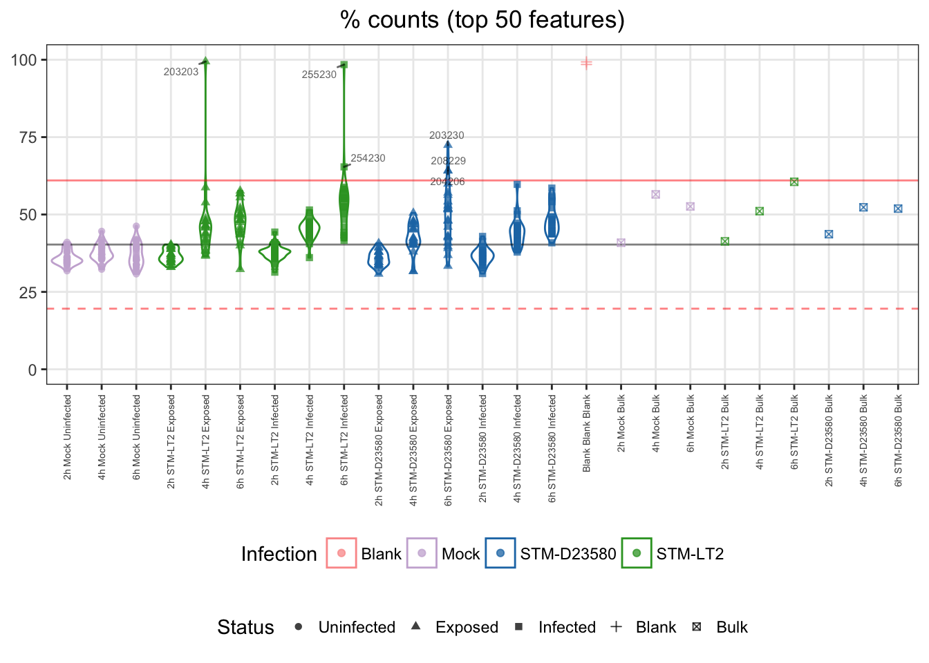
For reference:
- single cells
- median: 40%
- cut-off
- upper bound: 61%
100
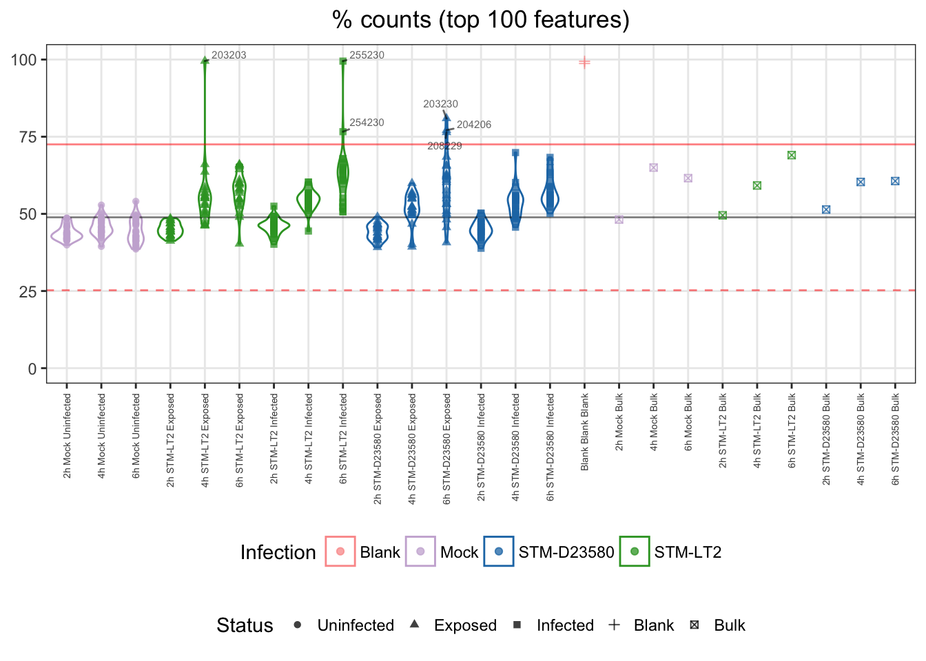
For reference:
- single cells
- median: 49%
- cut-off
- upper bound: 73%
Note: Two infected:D23580 samples appear near (below) the cut-off threshold. This observation can be related to the overall library complexity figure shown earlier.
200
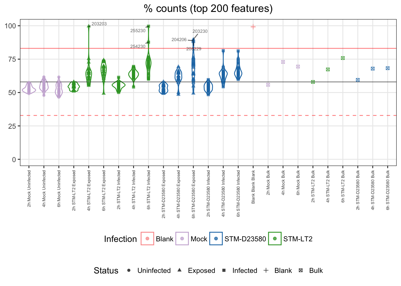
For reference:
- single cells
- median: 58%
- cut-off
- upper bound: 83%
Note: Two infected:D23580 samples appear near (below) the cut-off threshold. This observation can be related to the overall library complexity figure shown earlier.
Count of detected features
A notion closely related to library complexity is the count of features detected within each individual sample. Although the definition of “detection level” may be debated, we will consider here any feature with non-zero count.
Abnormal counts of detected features may be indicative of technical issue during RNA capture and library preparation; for instance, excessively low counts of detected features may indicate RNA degradation, while excessively high counts of detected features may indicate capture of multiple cells.
Owing to the considerable amount of variation that results from the relaxed definition of detection level above, let us apply a somewhat stringent cut-off of 2 MADs to identify as outliers single cells with a count of detected features excessively lower than the median of single cell samples, here beyond 2 MADs::
outliers$FeaturesCount <- isOutlier(sce.sc$total_features, 2, "lower")
table(outliers$FeaturesCount)
##
## FALSE TRUE
## 361 12Let us visualise outliers, along with blank and bulk samples, for reference:
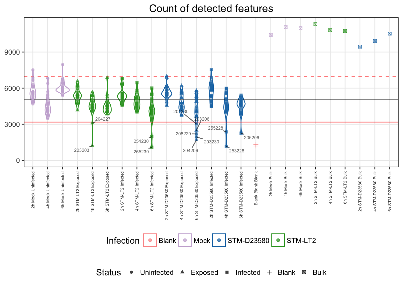
For reference:
- single cells
- median: 5068
- cut-offs
- lower bound: 3173.2
ERCC content
An identical–yet very small–quantity of ERCC spike-in features is added to each sample prior to library preparation. As a result, technical variation and issues during library preparation may be estimated from the proportion of reads assigned to those spike-in features; an excessive proportion of reads assigned to ERCC spike-in features may indicate eukaryotic RNA degradation, while excessive variation may indicate cDNA amplication bias.
Due to the limited amount of variation that results from the generally low levels of ERCC spike-in features detected, let us apply a somewhat relaxed cut-off of 5 MADs to identify as outliers single cells an ERCC content excessively higher than the median of single cell samples:
outliers$ERCC <- isOutlier(sce.sc$pct_counts_ERCC, 5, "higher")
table(outliers$ERCC)
##
## FALSE TRUE
## 357 16Let us visualise those outliers, along with blank and bulk samples for reference:
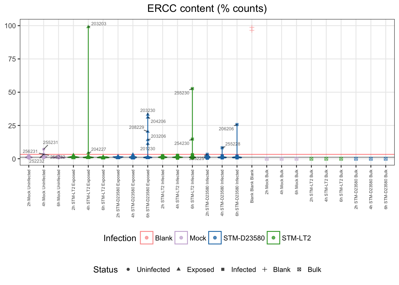
For reference:
- single cells
- median: 1%
- cut-offs
- upper bound: 3%
Mitochondrial content
Similarly to ERCC spike-in features, mitochondrial RNA may be used as an endogenous source of control features; the limited count of genes encoded on the mitochondrial chromosome relative to the human chromosomes implies that, even at their highest levels of expression, mitochondrial genes are expected to account for a low proportion of the total read count in each sample. Consequently, abnormally high proportions of reads assigned to mitochondrial gene features may be indicative of technical issue during RNA capture and library preparation, or abnormal count of mitochondria within the single cells.
Conversely, an unusually low proportion of reads assigned to mitochondrial gene features may also indicate issues related to RNA capture and library preparation.
Let us identify as outliers single cells for which the proportion of reads assigned to mitochondrial gene features is excessively higher than the median of single cell samples:
outliers$MT <- isOutlier(sce.sc$pct_counts_MT, 3, "higher")
table(outliers$MT)
##
## FALSE TRUE
## 362 11Let us visualise those outliers, along with blank and bulk samples for reference:
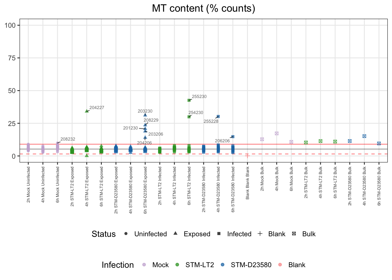
For reference:
- single cells
- median: 5%
- cut-offs
- upper bound: 11%
Summary
Let us display the count of cells identified as outliers for each of the filters in this section:
scater.fr <- FilterRules(setdiff(colnames(outliers), names(fastqc.fr)))
scater.fr
## FilterRules of length 6
## names(6): top50 top100 top200 FeaturesCount ERCC MT| Fail | Pass | |
|---|---|---|
| 373 | 373 | |
| top50 | 6 | 367 |
| top100 | 6 | 367 |
| top200 | 6 | 367 |
| FeaturesCount | 12 | 361 |
| ERCC | 16 | 357 |
| MT | 11 | 362 |
| 5 | 355 |
Global summary of QC metrics
By filter
Let us now collect the results of all the QC metrics obtained in the previous sections, and display the count of cells :
all.fr <- FilterRules(colnames(outliers))
all.fr
## FilterRules of length 10
## names(10): GC AlignedPercent AssignedCount ... FeaturesCount ERCC MT| Fail | Pass | |
|---|---|---|
| 373 | 373 | |
| GC | 1 | 372 |
| AlignedPercent | 20 | 353 |
| AssignedCount | 21 | 352 |
| AssignedPercent | 16 | 357 |
| top50 | 6 | 367 |
| top100 | 6 | 367 |
| top200 | 6 | 367 |
| FeaturesCount | 12 | 361 |
| ERCC | 16 | 357 |
| MT | 11 | 362 |
| 0 | 342 |
In the table above, none of the cells fails all the filters; this demonstrates the importance of each individual filter, despite the apparent relatedness and overlap between many of the metrics.
As a result, let us identify the cells that passed all of the above filters:
idx.pass <- (rowSums(evalSeparately(all.fr, outliers)) == 0)By cell
Secondly, we may also examine the count of single cell samples, according to the number of QC filters that they have failed:
| Filters | Cells |
|---|---|
| 0 | 342 |
| 1 | 13 |
| 2 | 2 |
| 3 | 5 |
| 5 | 1 |
| 6 | 4 |
| 9 | 6 |
By phenotype
We may summarise experimental phenotype information for the outliers samples, or alternatively, the samples that successfully passed all filters:
Outliers
summary(data.frame(colData(sce.sc))[
  !idx.pass,
  c("Infection", "Status", "Time", "Lane", "Plate")
])
## Infection Status Time Lane Plate
## Mock :11 Uninfected:11 2h: 5 305264:20 P1: 6
## STM-LT2 : 7 Exposed :11 4h:15 305265:11 P2:14
## STM-D23580:13 Infected : 9 6h:11 P3: 9
## P4: 2Passed
summary(data.frame(colData(sce.sc))[
  idx.pass,
  c("Infection", "Status", "Time", "Lane", "Plate")
])
## Infection Status Time Lane Plate
## Mock : 80 Uninfected: 80 2h:119 305264:165 P1:86
## STM-LT2 :134 Exposed :127 4h:110 305265:177 P2:79
## STM-D23580:128 Infected :135 6h:113 P3:86
## P4:91Heat map summary view
Let us define an order of sample that groups single cells by experimental phenotypes:
cells.order <- with(colData(sce.sc), order(Time, Status, Infection))We may then display the QC metrics failed by each single cell as red cells in an heat map:
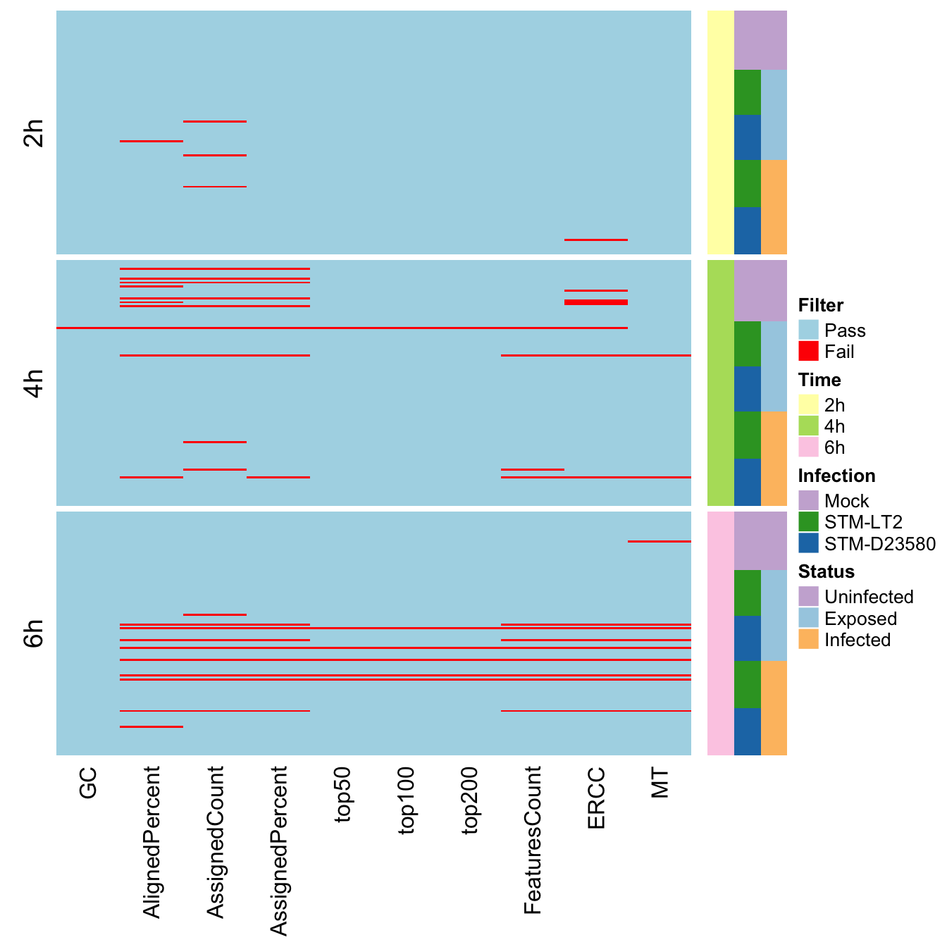
## quartz_off_screen
##                 2
## quartz_off_screen
## 2Single cells selection
Let us finally retain the single cells that passed all QC metrics into a new SCESet:
sce.pass <- sce.sc[,idx.pass]
dim(sce.pass)
## [1] 58084 342For each experimental groups, we may display the count of cells that passed the above QC are as follow, as well as the initial count of cells, for reference :
| Initial | Passed | Failed | Time | Infection | Status |
|---|---|---|---|---|---|
| 30 | 30 | 0 | 2h | Mock | Uninfected |
| 31 | 21 | 10 | 4h | Mock | Uninfected |
| 30 | 29 | 1 | 6h | Mock | Uninfected |
| 23 | 23 | 0 | 2h | STM-LT2 | Exposed |
| 23 | 21 | 2 | 4h | STM-LT2 | Exposed |
| 23 | 22 | 1 | 6h | STM-LT2 | Exposed |
| 24 | 23 | 1 | 2h | STM-LT2 | Infected |
| 24 | 23 | 1 | 4h | STM-LT2 | Infected |
| 24 | 22 | 2 | 6h | STM-LT2 | Infected |
| 23 | 20 | 3 | 2h | STM-D23580 | Exposed |
| 23 | 23 | 0 | 4h | STM-D23580 | Exposed |
| 23 | 18 | 5 | 6h | STM-D23580 | Exposed |
| 24 | 23 | 1 | 2h | STM-D23580 | Infected |
| 24 | 22 | 2 | 4h | STM-D23580 | Infected |
| 24 | 22 | 2 | 6h | STM-D23580 | Infected |