Sum factors

Having identified in previous sections:

cells with good quality sequencing data (here),
features detected in at least one of the experimental groups (here);

We may now normalise expression levels between cells using an approach suitable for single cell data sets.

Unsupervised clusters

Considering the multifactorial experimental design of this data set, and the considerable transcriptional changes expected over time, and in response to bacterial stimuli, let us first identify clusters of transcriptionally similar cells; those unsupervised clusters will subsequently be used to apply a stratified normalisation procedure within each cluster, concluded by a scaling of size factors for comparison between clusters, as implemented in the scran package.

Importantly, let us define the smallest cluster size to the minimum number of cells in any experimental group (i.e., 18 cells in group 6h_STM-D23580_Exposed; see this earlier section for the count of cells per group).

Note: The default behaviour of the quickCluster function is to only use endogenous features (get.spikes=FALSE), as ERCC spike-in features should be present in equal amounts in all samples:

clusters <- quickCluster(  sce.filtered, min.size=min(table(sce.filtered$Group)))
sce.filtered$Cluster <- clusters

Cluster	Cells
1	137
2	87
3	84
4	34

In this case, four clusters were identified. Let us examine the distribution of experimental groups across the identified clusters:

longCluster <- reshape2::melt(
  data.frame(colData(sce.filtered)[,c("Cluster","Time","Infection","Status")]),
  measure.vars = c("Time","Infection","Status"),
  variable.name = "Factor", value.name = "Level"
)
longCluster$Level <- with(
  colData(sce.filtered),
  factor(longCluster$Level, rev(c(levels(Time), levels(Infection), levels(Status))))
)

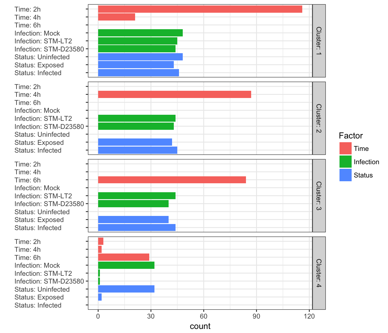
As expected, the figure above demonstrates that the largest cluster (cluster 1: 137 cells) contains most 2h cells and 4h:uninfected cells (which cannot be found in any other facet). Clusters 2 and 3 contain uniquely 4h and 6h stimulated cells, respectively. Finally, the smallest cluster (4) contains mostly 6h:uninfected, with a handful of other cells.

Compute size factors

Let us apply the normalisation procedure, deconvolving size factors clusters:

sce.filtered <- computeSumFactors(
  sce.filtered, sizes = c(10, 15), clusters = sce.filtered$Cluster)
ggplot(data.frame(colData(sce.filtered, internal=TRUE))) +
  geom_histogram(
    aes(size_factor, fill=Time),
    binwidth = 0.1, colour="black", position = position_stack()) +
  scale_x_continuous(limits = c(0, 2)) +
  labs(x = "Size factor") +
  theme_bw()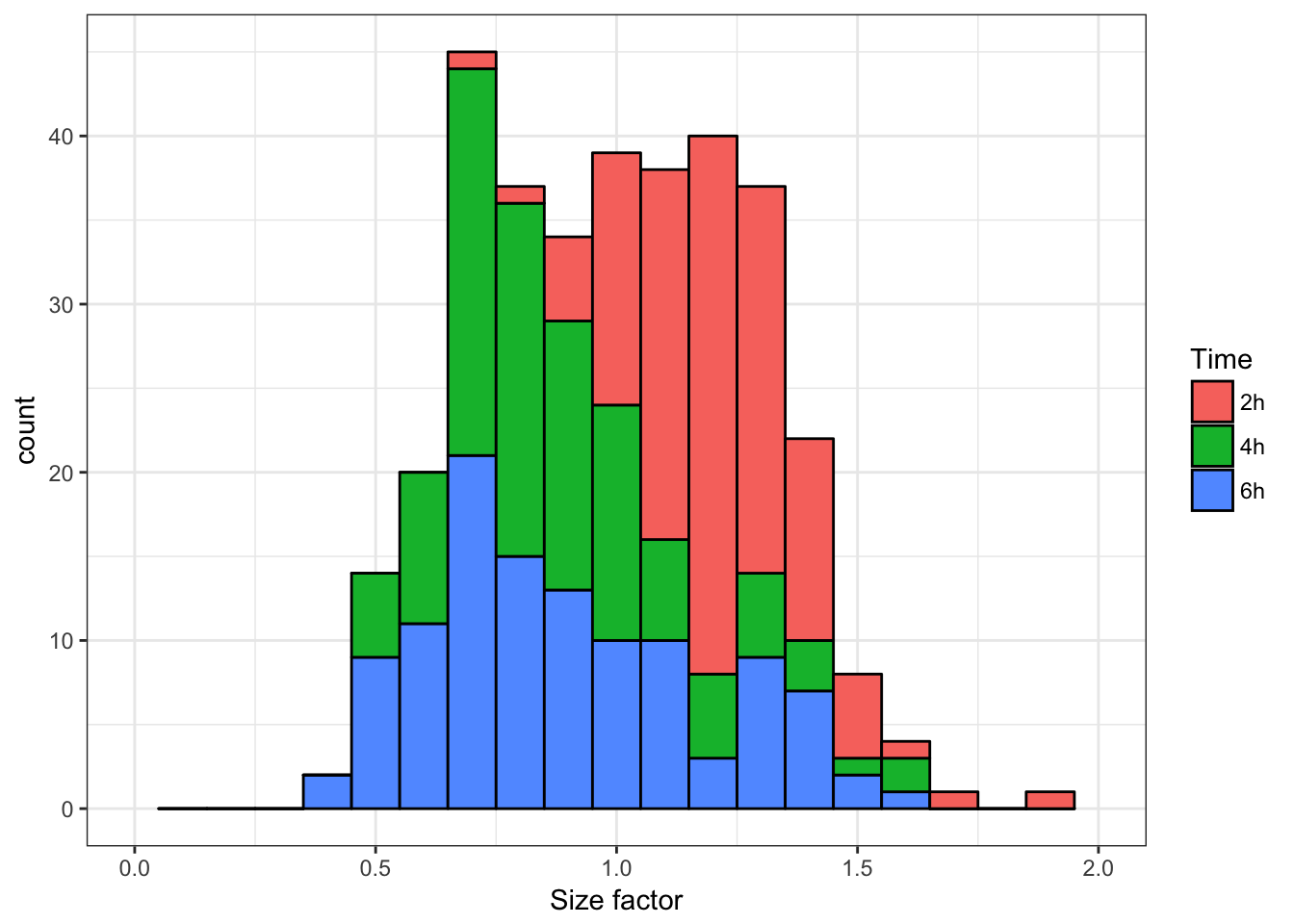

Relation to library size

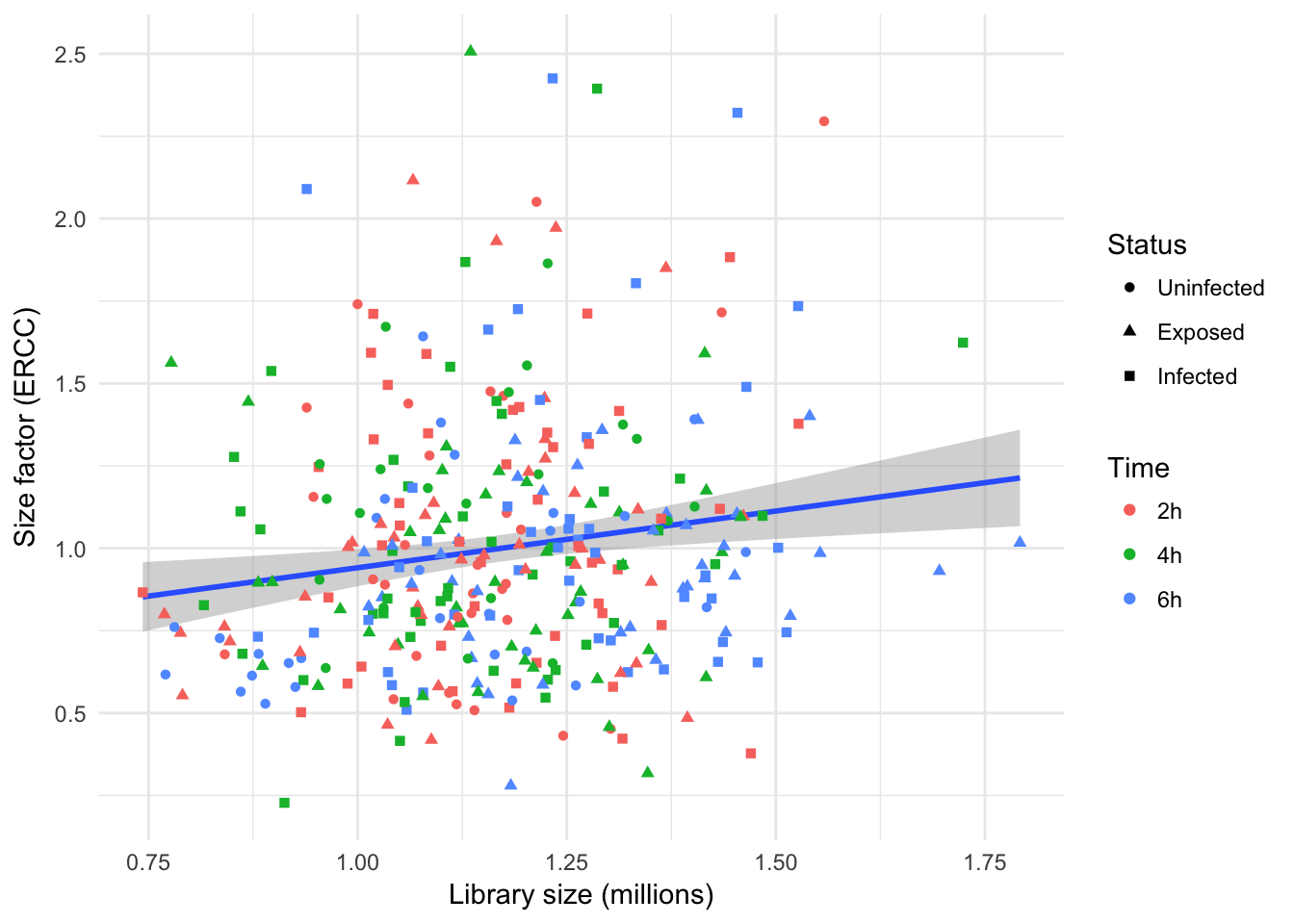
In the absence of biological effect, size factors are expected to correlate with library size (Lun, McCarthy, and Marioni 2016). Let us visualise the two values in a scatter plot:

Scatter: Status

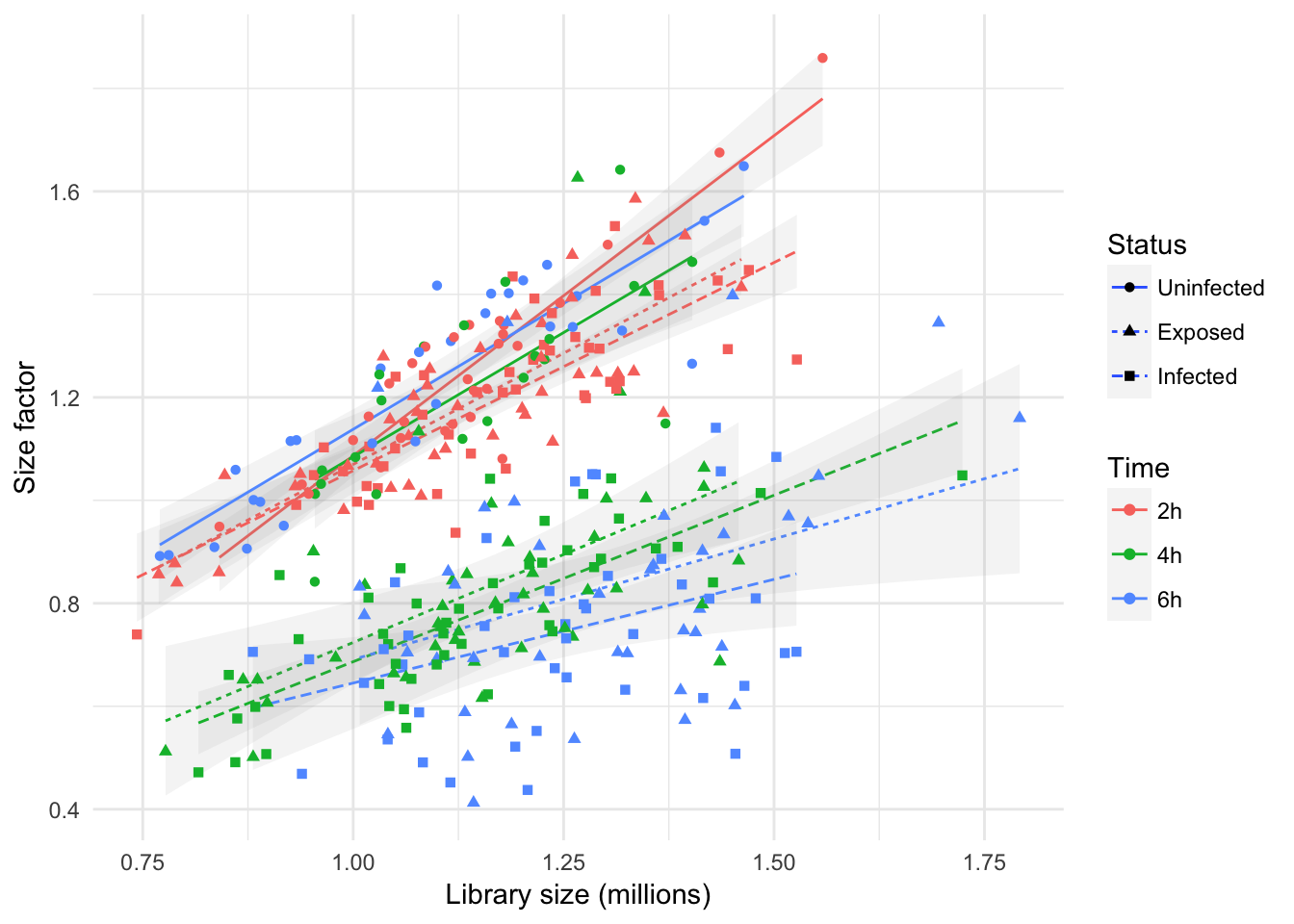
In the figure above, the size factors are somewhat correlated with library size, while significant scatter is visible around the trend; augmenting the figure with experimental phenotype information emphasises how the effect of library size on the size factor of individual cells is subject to factors related to the experimental design of the experiment.

In particular, the figure emphasises how the effect of library size is more important in uninfected cells, and at the earliest time point (i.e., 2h), when the biological effect of infection may not have fully affect the transcriptome of most cells yet.

In contrast, at later time points (i.e., 4h and 6h), trends indicate a markedly weaker effect of library size on size factor.

This suggest that other sources of systematic differences between cells arose (i.e., Status, Infection), and that differential expression is to be expected between experimental groups at those time points

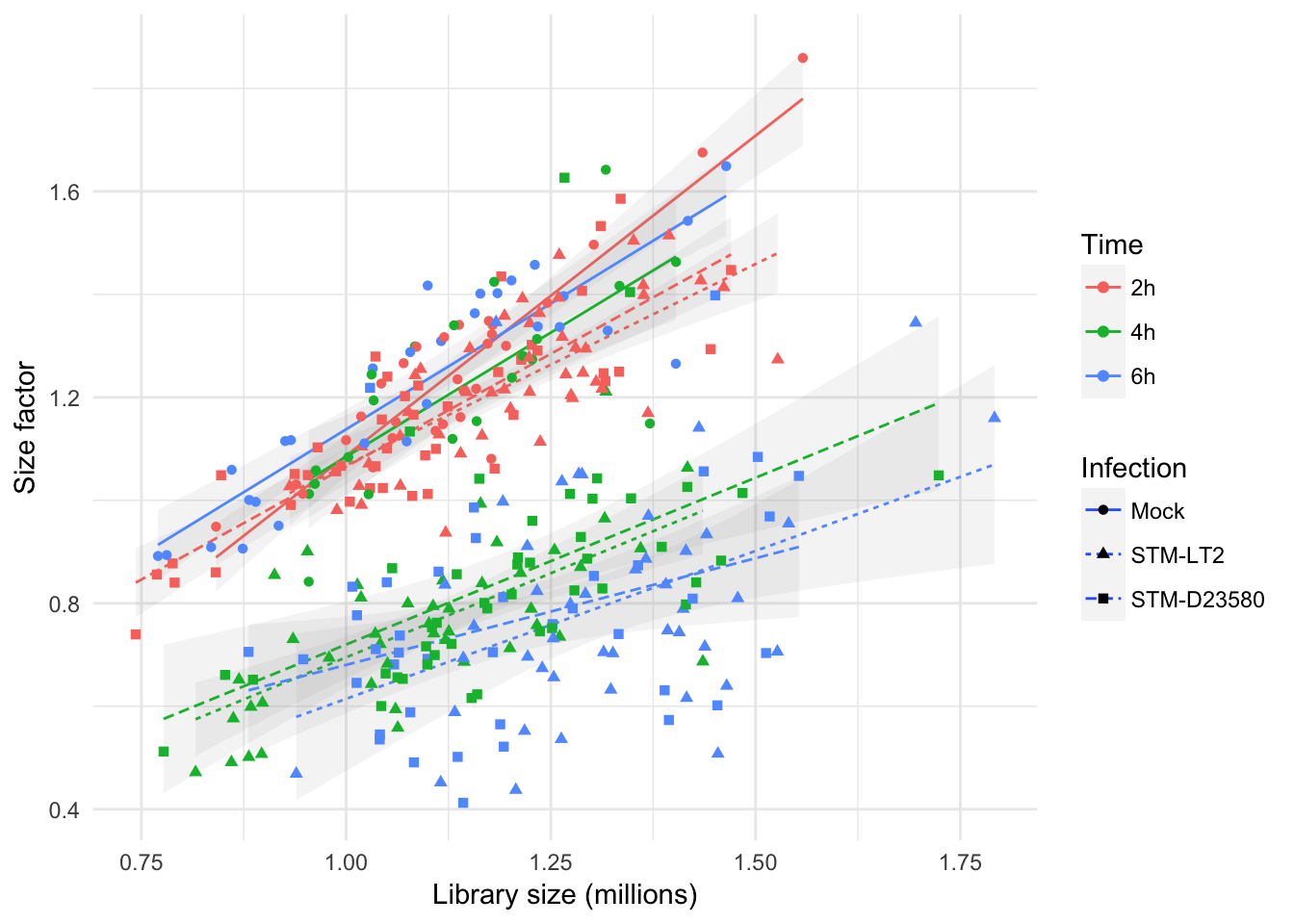
Scatter: Infection

Relation to experimental groups

The same effect to experimental covariates on the distribution of size factors within each experimental group may also be summarised in box plots as shown below:

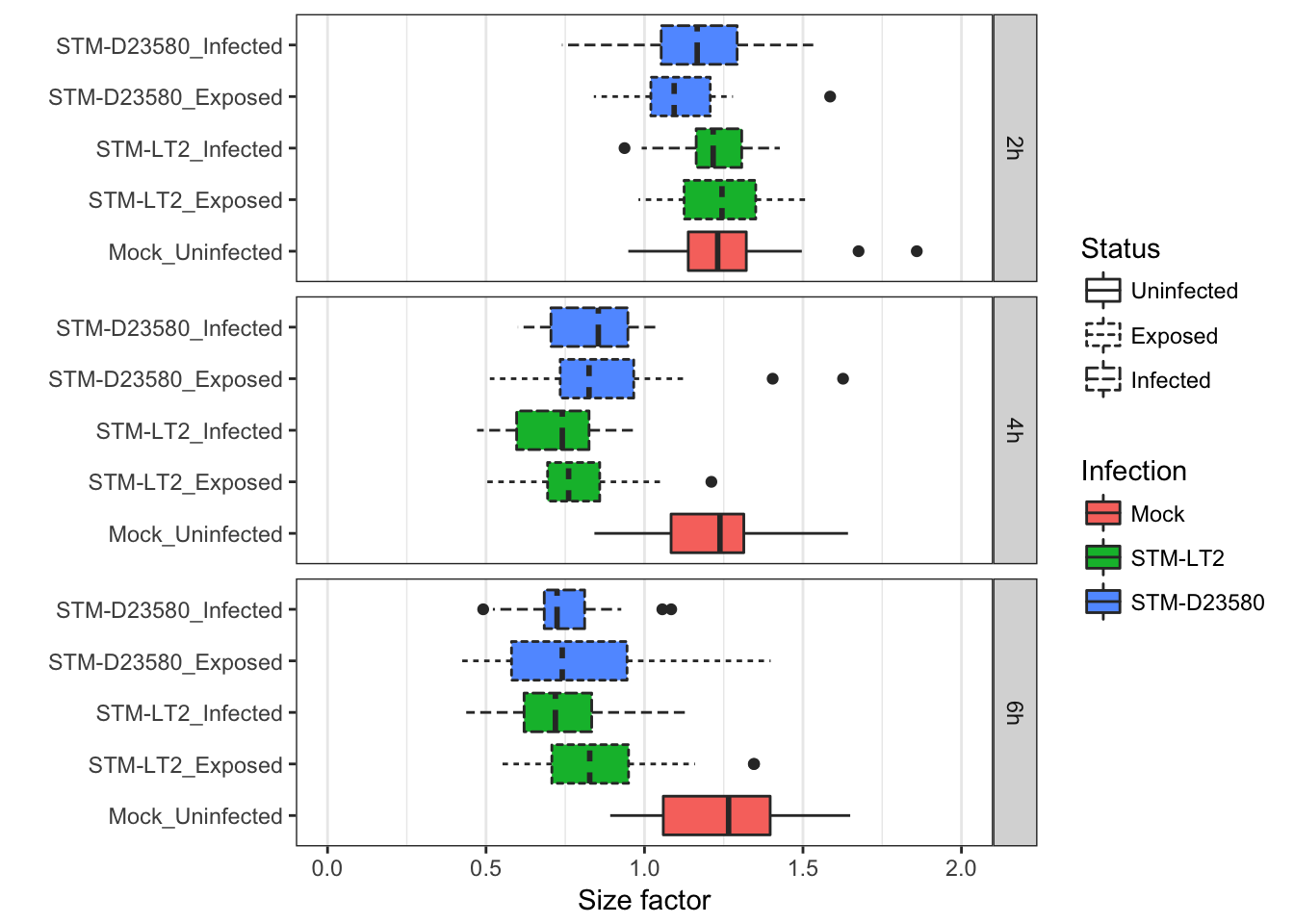
In a different perspective, the above figure emphasises again how size factors are affected by experimental factors in this data set; in particular at the later time points, size factors for cells stimulated with bacteria display markedly distinct size factors, irrespective of library size.

Overall, size factors suggest that experimental factors drive more important systematic differences between cells than library size at those time points, having likely reshaped the transcriptional profile of stimulated cells.

Spike factors

To ensure normalization is performed correctly, let us compute a separate set of size factors for the spike-in set. This assumes that none of the spike-in transcripts are differentially expressed.

sce.filtered <- computeSpikeFactors(
  sce.filtered, type = "ERCC", general.use = FALSE
)

We may then examine the spike factors calculated:

In contrast to the earlier size factors calculated using endogenous features, spike factors calculated using ERCC spike-in display a much weaker correlation with library size, and no trend with experimental factors.

Furthermore, this reinforces the absence of extreme outliers after the removal of cells with abnormal ERCC content in an earlier section; moreover, it suggests that counts assigned to individual ERCC spike-in features are similar across all the cells retained after quality control.

Apply size factors to normalise

The count data are used to compute normalized log-expression values for use in downstream analyses. Each value is defined as the log-ratio of each count to the size factor for the corresponding cell, after adding a prior count of 1 to avoid undefined values at zero counts. Division by the size factor ensures that any cell-specific biases are removed. Spike-in-specific size factors present are applied to normalize the spike-in transcripts separately from the endogenous features:

sce.norm <- normalize(sce.filtered)
assayNames(sce.norm)

## [1] "counts"    "cpm"       "logcounts"

References

Lun, A. T., D. J. McCarthy, and J. C. Marioni. 2016. “A Step-by-Step Workflow for Low-Level Analysis of Single-Cell Rna-Seq Data with Bioconductor.” Journal Article. F1000Res 5: 2122. doi:10.12688/f1000research.9501.2.

Normalisation