BiocPkgTools
Motivation
There are currently 6,096 packages on Bioconductor, broken down as follows:
| Repository | Packages |
|---|---|
| data-annotation | 2,693 |
| data-experiment | 855 |
| software | 2,516 |
| workflows | 32 |
In an effort to motivate myself to keep an eye out for interesting packages - both new and old - I have used the BiocPkgTools package to develop a website updated daily and feature packages selected randomly from each repository.
I have then set up a GitHub Action executed as a CRON job to update the website daily.
The result is accessible at: https://kevinrue.github.io/BiocRoulette/.
Example usage
Below, I include a bit of code that I wrote while developing the website, to illustrate the process.
First, the packages that I used to fetch, process, and visualise the data.
library(BiocPkgTools)
library(tidyverse)
library(cowplot)
Then I fetch the data using BiocPkgTools::biocDownloadStats().
download_stats <- biocDownloadStats()Next, I subset the download stats to a given repository.
software_stats <- download_stats %>% filter(pkgType == "software")Then, I identify the latest complete month with data in the download statistics. To do that, I look for the latest month with non-zero download statistics, and I take the month before that one.
latest_full_date <- software_stats %>%
  group_by(Date) %>%
  summarise(Nb_of_downloads = sum(Nb_of_downloads)) %>%
  filter(Nb_of_downloads > 0) %>%
  arrange(desc(Date)) %>%
  head(2) %>%
  tail(1) %>%
  pull(Date)
software_monthly_stats <- software_stats %>%
  filter(Date == latest_full_date)
I wanted to give an edge to packages more frequently downloaded, but without being overwhelmed by core packages that have excessively large download statistics.
To do so, I visualised the distribution of download stats, and I chose to weigh packages by the log(x+1) transformation of the number of distinct IP addresses in their download statistics.
gg_dl <- ggplot(software_monthly_stats) +
  geom_histogram(aes(Nb_of_downloads), color = "black", fill = "grey", size = 0.1) +
  scale_x_log10() +
  theme_cowplot() +
  labs(
    title = sprintf("%s %s", software_monthly_stats$Month, software_monthly_stats$Year)
  )
gg_ip <- ggplot(software_monthly_stats) +
  geom_histogram(aes(Nb_of_distinct_IPs), color = "black", fill = "grey", size = 0.1) +
  scale_x_log10() +
  theme_cowplot()
plot_grid(gg_dl, gg_ip, nrow = 1)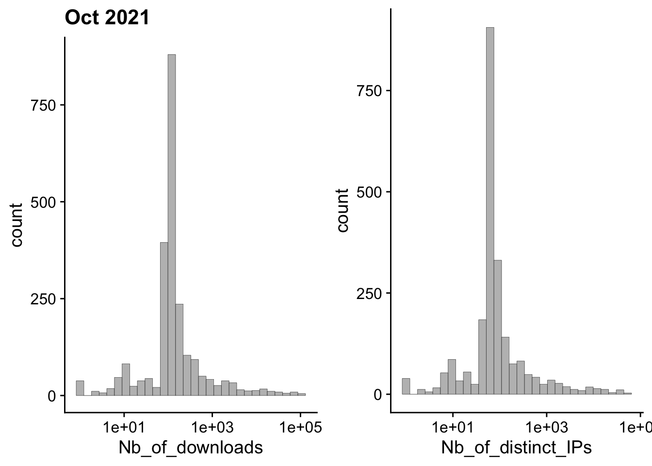
Finally, I set the random seed using the date of the day, and I randomly sample a package from the table, using the weight described above.
set.seed(as.numeric(Sys.Date()))
software_monthly_stats %>%
  sample_n(size = 1, replace = FALSE, weight = log(Nb_of_distinct_IPs + 1))
## # A tibble: 1 × 7
## pkgType Package Year Month Nb_of_distinct_IPs Nb_of_downloads Date
## <chr> <chr> <int> <chr> <int> <int> <date>
## 1 software Qtlizer 2021 Oct 51 92 2021-10-01