The predict method

The basesets object can immediately be supplied to the predict S3 method, in combination with the SummarizedExperiment object to annotate. However, the cell type signatures described in the Seurat - Guided Clustering Tutorial use gene symbol identifiers, which do not match the Ensembl gene identifiers used in rownames(sce). Here, to make the gene identifiers compatible between the data set and the signatures, we simply replace the Ensembl gene identifiers by the "Symbol_TENx" gene metadata, after making duplicated values unique.

library(hancock)
rownames(sce) <- make.unique(rowData(sce)[["Symbol_TENx"]])
sce <- predict(basesets, sce, method="ProportionPositive", cluster.col="seurat.ident")

Prediction outputs

The updated SummarizedExperiment object is returned, with a number of additional metadata.

The key output is the cell identity predicted for each cell in the object. This information is stored in colData(sce)[["hancock"]][["prediction"]], or sce$hancock$prediction, in short.

table(sce$hancock$prediction)

## 
##       CD4 T cells   CD14+ Monocytes           B cells       CD8 T cells 
##              1151               479               342               308 
## FCGR3A+ Monocytes          NK cells   Dendritic Cells    Megakaryocytes 
##               157               155                32                14

With method="ProportionPositive", all cells in each cluster are annotated with the predominant signature in their associated cluster. As such, the cell type prediction may be tabulated against the cluster membership of each cell. This view can potentially highlight multiple clusters labelled by the same predicted label as a sign of overclustering.

table(sce$hancock$prediction, sce$seurat.ident)

##                    
##                        0    1    2    3    4    5    6    7
##   CD4 T cells       1151    0    0    0    0    0    0    0
##   CD14+ Monocytes      0  479    0    0    0    0    0    0
##   B cells              0    0  342    0    0    0    0    0
##   CD8 T cells          0    0    0  308    0    0    0    0
##   FCGR3A+ Monocytes    0    0    0    0  157    0    0    0
##   NK cells             0    0    0    0    0  155    0    0
##   Dendritic Cells      0    0    0    0    0    0   32    0
##   Megakaryocytes       0    0    0    0    0    0    0   14

In addition to the final predictions, the updated SummarizedExperiment object also contain some additional information tracing to the process of prediction. That information can be found in metadata(sce)[["hancock"]].

names(metadata(sce)[["hancock"]])

## [1] "GeneSets"                    "method"                     
## [3] "packageVersion"              "ProportionPositiveByCluster"
## [5] "TopSignatureByCluster"

In particular:

• GeneSets stores the object that provided the gene set signatures used for the prediction
• method stores the name of the method used to make the predictions
• packageVersion stores the version of the hancock package used to make the predictions

Specifically, method="ProportionPositive" adds the following metadata items:

• ProportionPositiveByCluster stores the matrix indicating the proportion of cells in each cluster that are positive for each signature
• TopSignatureByCluster stores a named vector that indicates the predominant signature for each cluster. It is shown below.

metadata(sce)[["hancock"]][["TopSignatureByCluster"]]

##                 0                 1                 2                 3 
##       CD4 T cells   CD14+ Monocytes           B cells       CD8 T cells 
##                 4                 5                 6                 7 
## FCGR3A+ Monocytes          NK cells   Dendritic Cells    Megakaryocytes 
## 8 Levels: CD4 T cells CD14+ Monocytes B cells ... Megakaryocytes

Heat map

It is possible to visualize the proportion of cells positive for each signature in each cluster as a heat map. Note how the diagonal (displaying the tutorial annotations) shows high proportions of cells matching the annotated signature.

plotProportionPositive(sce, cluster_rows=FALSE, cluster_columns=FALSE)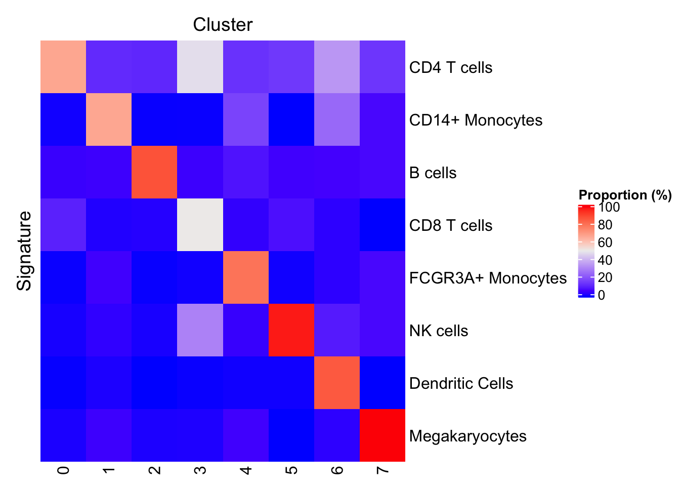

We can also let signatures and clusters of cells cluster in the heat map. Unsurprisingly, the subpopulations of monocytes show some similarity, as do the subpopulations of CD4 positive and CD8 positive T cells.

plotProportionPositive(sce)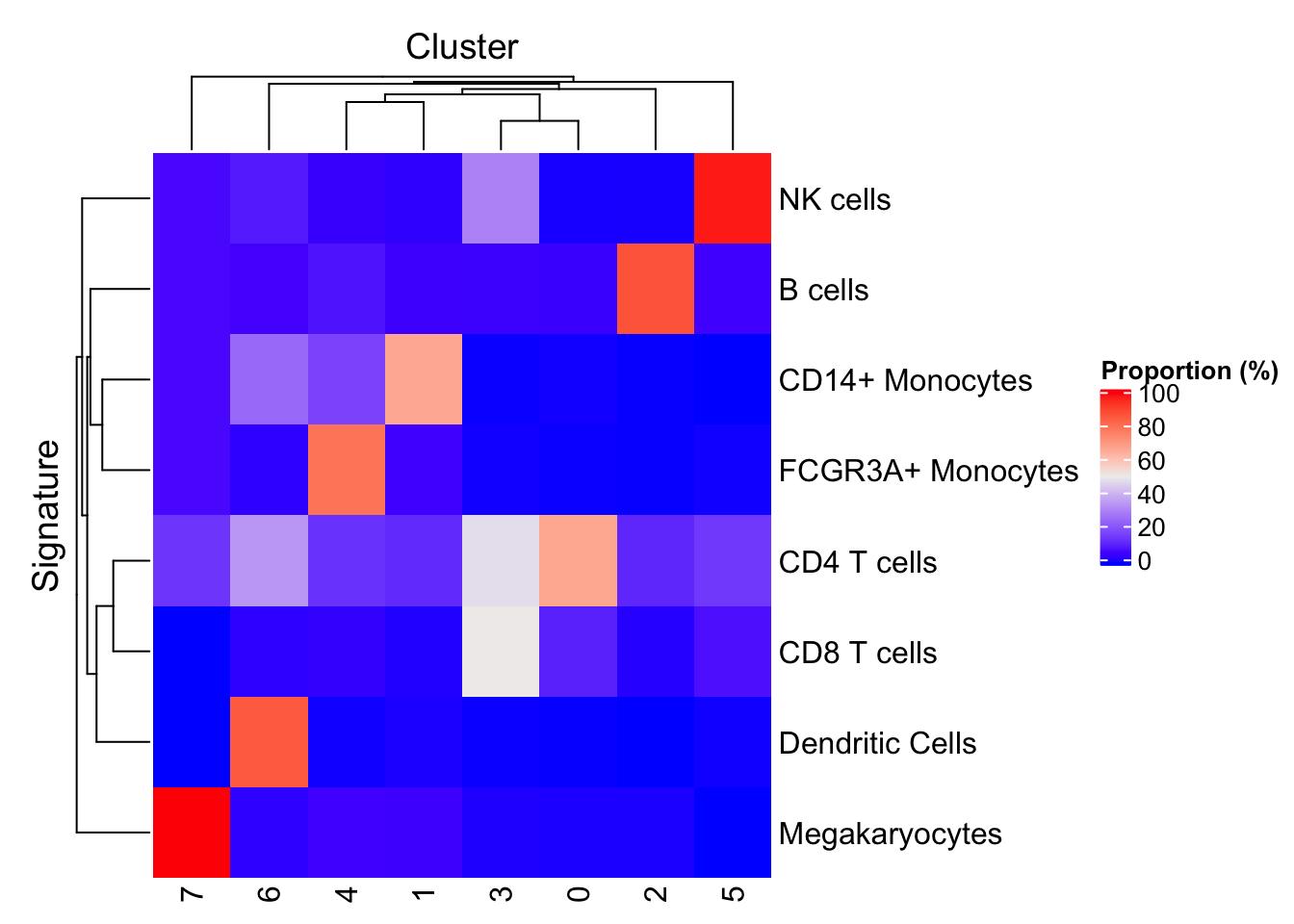

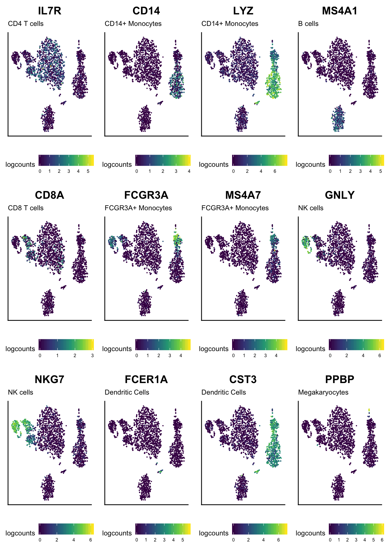
Reduced dimension

With a bit more code, we can also display the expression of each marker on the result of t-SNE dimensionality reduction.

library(ggplot2)
library(cowplot)
ggList <- list()
for (markerName in ids(elementInfo(basesets))) {
    ggDataFrame <- data.frame(
        reducedDim(sce, "TSNE"),
        logcounts=log2(assay(sce, "counts")[markerName, ] + 1)
    )
    cellIdentity <- subset(as.data.frame(basesets), element == markerName, "set", drop=TRUE)
    gg <- ggplot(ggDataFrame, aes(tSNE_1, tSNE_2, color=logcounts)) +
        geom_point(size=0.1) +
        scale_color_viridis_c() +
        labs(title=markerName, subtitle=cellIdentity, x=NULL, y=NULL) +
        theme(
            axis.text = element_blank(), axis.ticks = element_blank(),
            text = element_text(size=rel(3)), legend.text = element_text(size=rel(2)),
            legend.position = "bottom")
    ggList[[markerName]] <- gg
}
cowplot::plot_grid(plotlist = ggList)