Spotify Yourself
Kevin Rue-Albrecht
MRC WIMM Centre for Computational Biology, University of Oxford, Oxford, OX3 9DS, UKkevinrue67@gmail.com
16 July 2025
Source:vignettes/kevin.Rmd
kevin.RmdCompiled date: 2025-07-16
Last edited: 2020-04-20
License: MIT + file LICENSE
Introduction
spotify is an R package.
Once installed, the package can be loaded and attached to your current workspace as follows:
Other helpful libraries.
Demonstration
Input file
input_file <- system.file(package = "spotify", "Kevin.jpg")Output types
Raw image
kevin <- spotify(
  path = input_file
)
print(kevin)
#> # A tibble: 1 × 7
#>   format width height colorspace matte filesize density
#>   <chr>  <int>  <int> <chr>      <lgl>    <int> <chr>
#> 1 WEBP    1140   1140 sRGB       FALSE    69414 72x72
Flattened image
kevin <- spotify(
  path = input_file,
  return.type = "flatten",
  extras = list(
    image_flatten = list(operator = "Modulate")
  )
)
print(kevin)
#> # A tibble: 1 × 7
#>   format width height colorspace matte filesize density
#>   <chr>  <int>  <int> <chr>      <lgl>    <int> <chr>
#> 1 WEBP    1140   1140 sRGB       FALSE        0 72x72
Image data
kevin <- spotify(
  path = input_file,
  return.type = "data"
)
kevin
#> 3 channel 1140x1140 bitmap array: 'bitmap' raw [1:3, 1:1140, 1:1140] ff ff ff ff ...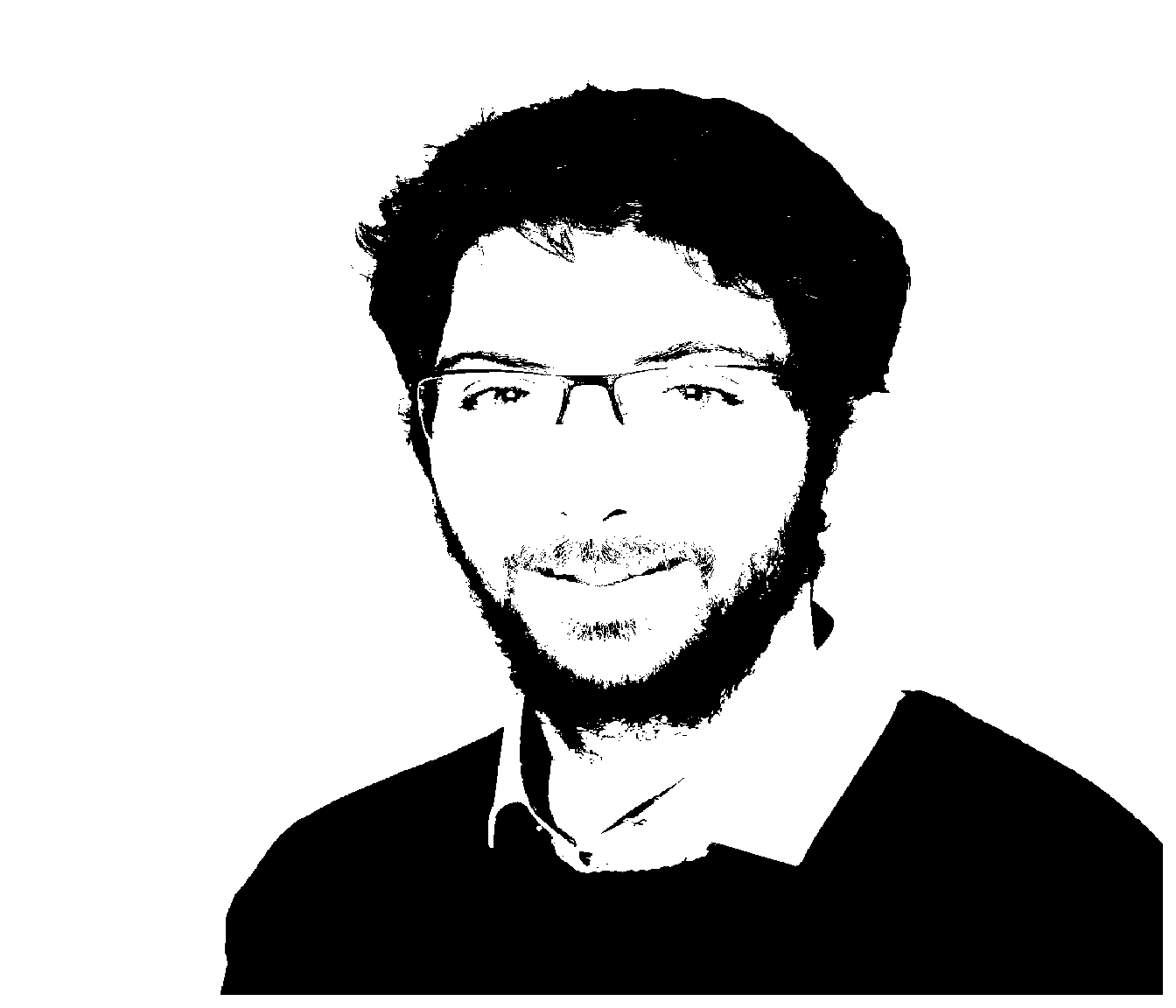

Jittered scatter plot
spotify(
  path = input_file,
  return.type = "jitter",
  downsample = 100,
  jitter = 5
) + theme_void()
Xenium-like
spotify(
  path = input_file,
  return.type = "spatial",
  downsample = 75,
  jitter = 5,
  extras = list(
    cluster = list(k.nn = 50, k.cluster = 10)
  )
) + theme_void() + guides(colour = "none")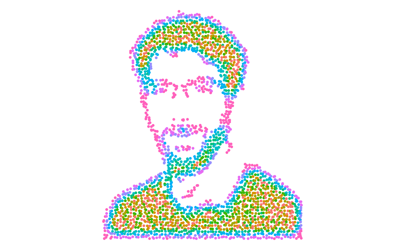
Visium-like
spotify(
  path = input_file,
  return.type = "visium",
  downsample = 100,
  point.size = 0.25,
  extras = list(
    cluster = list(k.nn = 50, k.cluster = 10)
  )
) + theme_void() + guides(colour = "none")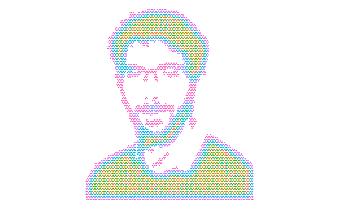
Additional information
The GitHub repository contains the development version of the package, where new functionality is added over time. The authors appreciate well-considered suggestions for improvements or new features, or even better, pull requests.
If you use spotify for your analysis, please cite it as shown below:
citation("spotify")
#> To cite package 'spotify' in publications use:
#>
#>   Rue-Albrecht K (2024). _spotify: Spotify Your Images_. R package
#>   version 0.1.0, <https://kevinrue.github.io/spotify>.
#>
#> A BibTeX entry for LaTeX users is
#>
#>   @Manual{,
#>     title = {spotify: Spotify Your Images},
#>     author = {Kevin Rue-Albrecht},
#>     year = {2024},
#>     note = {R package version 0.1.0},
#>     url = {https://kevinrue.github.io/spotify},
#>   }
Session Info
sessionInfo()
#> R version 4.5.1 (2025-06-13)
#> Platform: x86_64-pc-linux-gnu
#> Running under: Ubuntu 24.04.2 LTS
#>
#> Matrix products: default
#> BLAS:   /usr/lib/x86_64-linux-gnu/openblas-pthread/libblas.so.3
#> LAPACK: /usr/lib/x86_64-linux-gnu/openblas-pthread/libopenblasp-r0.3.26.so;  LAPACK version 3.12.0
#>
#> locale:
#>  [1] LC_CTYPE=en_US.UTF-8       LC_NUMERIC=C
#>  [3] LC_TIME=en_US.UTF-8        LC_COLLATE=en_US.UTF-8
#>  [5] LC_MONETARY=en_US.UTF-8    LC_MESSAGES=en_US.UTF-8
#>  [7] LC_PAPER=en_US.UTF-8       LC_NAME=C
#>  [9] LC_ADDRESS=C               LC_TELEPHONE=C
#> [11] LC_MEASUREMENT=en_US.UTF-8 LC_IDENTIFICATION=C
#>
#> time zone: UTC
#> tzcode source: system (glibc)
#>
#> attached base packages:
#> [1] stats     graphics  grDevices utils     datasets  methods   base
#>
#> other attached packages:
#> [1] ggplot2_3.5.2    spotify_0.1.0    BiocStyle_2.36.0
#>
#> loaded via a namespace (and not attached):
#>   [1] rlang_1.1.6                 magrittr_2.0.3
#>   [3] shinydashboard_0.7.3        clue_0.3-66
#>   [5] GetoptLong_1.0.5            matrixStats_1.5.0
#>   [7] compiler_4.5.1              mgcv_1.9-3
#>   [9] png_0.1-8                   systemfonts_1.2.3
#>  [11] vctrs_0.6.5                 pkgconfig_2.0.3
#>  [13] shape_1.4.6.1               crayon_1.5.3
#>  [15] fastmap_1.2.0               magick_2.8.7
#>  [17] XVector_0.48.0              labeling_0.4.3
#>  [19] fontawesome_0.5.3           utf8_1.2.6
#>  [21] promises_1.3.3              rmarkdown_2.29
#>  [23] UCSC.utils_1.4.0            shinyAce_0.4.4
#>  [25] ragg_1.4.0                  xfun_0.52
#>  [27] cachem_1.1.0                GenomeInfoDb_1.44.0
#>  [29] jsonlite_2.0.0              listviewer_4.0.0
#>  [31] later_1.4.2                 DelayedArray_0.34.1
#>  [33] parallel_4.5.1              cluster_2.1.8.1
#>  [35] R6_2.6.1                    bslib_0.9.0
#>  [37] RColorBrewer_1.1-3          GenomicRanges_1.60.0
#>  [39] jquerylib_0.1.4             Rcpp_1.1.0
#>  [41] bookdown_0.43               SummarizedExperiment_1.38.1
#>  [43] iterators_1.0.14            knitr_1.50
#>  [45] IRanges_2.42.0              httpuv_1.6.16
#>  [47] Matrix_1.7-3                splines_4.5.1
#>  [49] igraph_2.1.4                tidyselect_1.2.1
#>  [51] abind_1.4-8                 yaml_2.3.10
#>  [53] doParallel_1.0.17           codetools_0.2-20
#>  [55] miniUI_0.1.2                lattice_0.22-7
#>  [57] tibble_3.3.0                withr_3.0.2
#>  [59] Biobase_2.68.0              shiny_1.11.1
#>  [61] evaluate_1.0.4              desc_1.4.3
#>  [63] circlize_0.4.16             pillar_1.11.0
#>  [65] BiocManager_1.30.26         MatrixGenerics_1.20.0
#>  [67] DT_0.33                     foreach_1.5.2
#>  [69] stats4_4.5.1                shinyjs_2.1.0
#>  [71] generics_0.1.4              dbscan_1.2.2
#>  [73] iSEE_2.20.0                 S4Vectors_0.46.0
#>  [75] scales_1.4.0                xtable_1.8-4
#>  [77] glue_1.8.0                  tools_4.5.1
#>  [79] colourpicker_1.3.0          fs_1.6.6
#>  [81] grid_4.5.1                  colorspace_2.1-1
#>  [83] SingleCellExperiment_1.30.1 nlme_3.1-168
#>  [85] GenomeInfoDbData_1.2.14     vipor_0.4.7
#>  [87] cli_3.6.5                   textshaping_1.0.1
#>  [89] viridisLite_0.4.2           S4Arrays_1.8.1
#>  [91] ComplexHeatmap_2.24.1       dplyr_1.1.4
#>  [93] gtable_0.3.6                rintrojs_0.3.4
#>  [95] sass_0.4.10                 digest_0.6.37
#>  [97] BiocGenerics_0.54.0         SparseArray_1.8.0
#>  [99] ggrepel_0.9.6               rjson_0.2.23
#> [101] htmlwidgets_1.6.4           farver_2.1.2
#> [103] htmltools_0.5.8.1           pkgdown_2.1.3
#> [105] lifecycle_1.0.4             shinyWidgets_0.9.0
#> [107] httr_1.4.7                  GlobalOptions_0.1.2
#> [109] mime_0.13