Compute Metagenes for Lists of Samples and Gene Sets

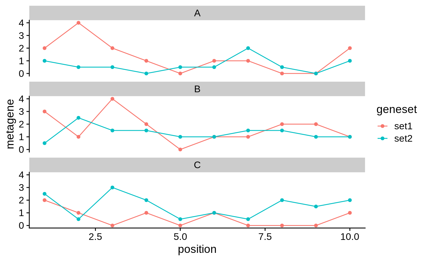
This function takes a list of data sets stratified by samples and gene sets. It computes the metagene for each gene set in each sample, and returns a data.frame suitable for ggplot2::ggplot().

makeMetageneDataFrame(list, assay.type = "matrix")

Arguments

list	A named list of lists of SummarizedExperiment objects. Each item in the top-most list is a named sample (e.g. "replicate1"). Each item within each sublist is a named gene set (e.g. "upregulated"). Each SummarizedExperiment object stores matrix of histone modification enrichment, with colnames indicating the index or coordinate of bins used to compute enrichment.
assay.type	Name the assay to average between all samples.

Value

A data.frame with columns named:

• "sample"

• "geneset"

• "position"

See also

importDeeptoolsExperiment

Examples

# Set the plotting environment ----

library(ggplot2)
library(cowplot)
#> 
#> ********************************************************
#> Note: As of version 1.0.0, cowplot does not change the
#>   default ggplot2 theme anymore. To recover the previous
#>   behavior, execute:
#>   theme_set(theme_cowplot())
#> ********************************************************
theme_set(theme_cowplot())

# Prepare example data ----

sample_names <- c("A", "B", "C")

se_list <- generateDeeptoolsExperiments(20, 10, sample_names)
se_list
#> $A
#> class: RangedSummarizedExperiment 
#> dim: 20 10 
#> metadata(0):
#> assays(1): matrix
#> rownames(20): GR_1 GR_2 ... GR_19 GR_20
#> rowData names(0):
#> colnames(10): 1 2 ... 9 10
#> colData names(0):
#> 
#> $B
#> class: RangedSummarizedExperiment 
#> dim: 20 10 
#> metadata(0):
#> assays(1): matrix
#> rownames(20): GR_1 GR_2 ... GR_19 GR_20
#> rowData names(0):
#> colnames(10): 1 2 ... 9 10
#> colData names(0):
#> 
#> $C
#> class: RangedSummarizedExperiment 
#> dim: 20 10 
#> metadata(0):
#> assays(1): matrix
#> rownames(20): GR_1 GR_2 ... GR_19 GR_20
#> rowData names(0):
#> colnames(10): 1 2 ... 9 10
#> colData names(0):
#> 

# Split each sample into gene subsets ----

range_sets <- list(set1=c("GR_1"), set2=c("GR_2", "GR_3"))
se_list_list <- lapply(se_list, splitByGeneSet, range_sets)

# Usage ----

x <- makeMetageneDataFrame(se_list_list)

ggplot(x, aes(position, metagene, color=geneset)) +
    geom_line(aes(group=interaction(geneset, sample))) +
    geom_point() +
    facet_wrap(~sample, ncol=1)